aRt-o Pollo

Imagine a universe stranger than ours in which light has a peculiar property. Rather than diffusing its intensity with distance, and simply increasing it with multiple sources, light in this universe is different. When two light beams meet, their combined intensity depends on the angle between them. Right angles are the best - when two light beams meet at a point perpendicularly, they have the highest possible intensity at that point. As the angle becomes smaller or bigger than 90 degrees (pi/2 radians), the intensity becomes weaker.

Why would you imagine such a thing? I don’t know why I wonder about such things, but I often do. As an example, I drew the image below while thinking about this - we have two “suns”, the red dots are 90 degree intersections, the blue points are intersections with a smaller angle.

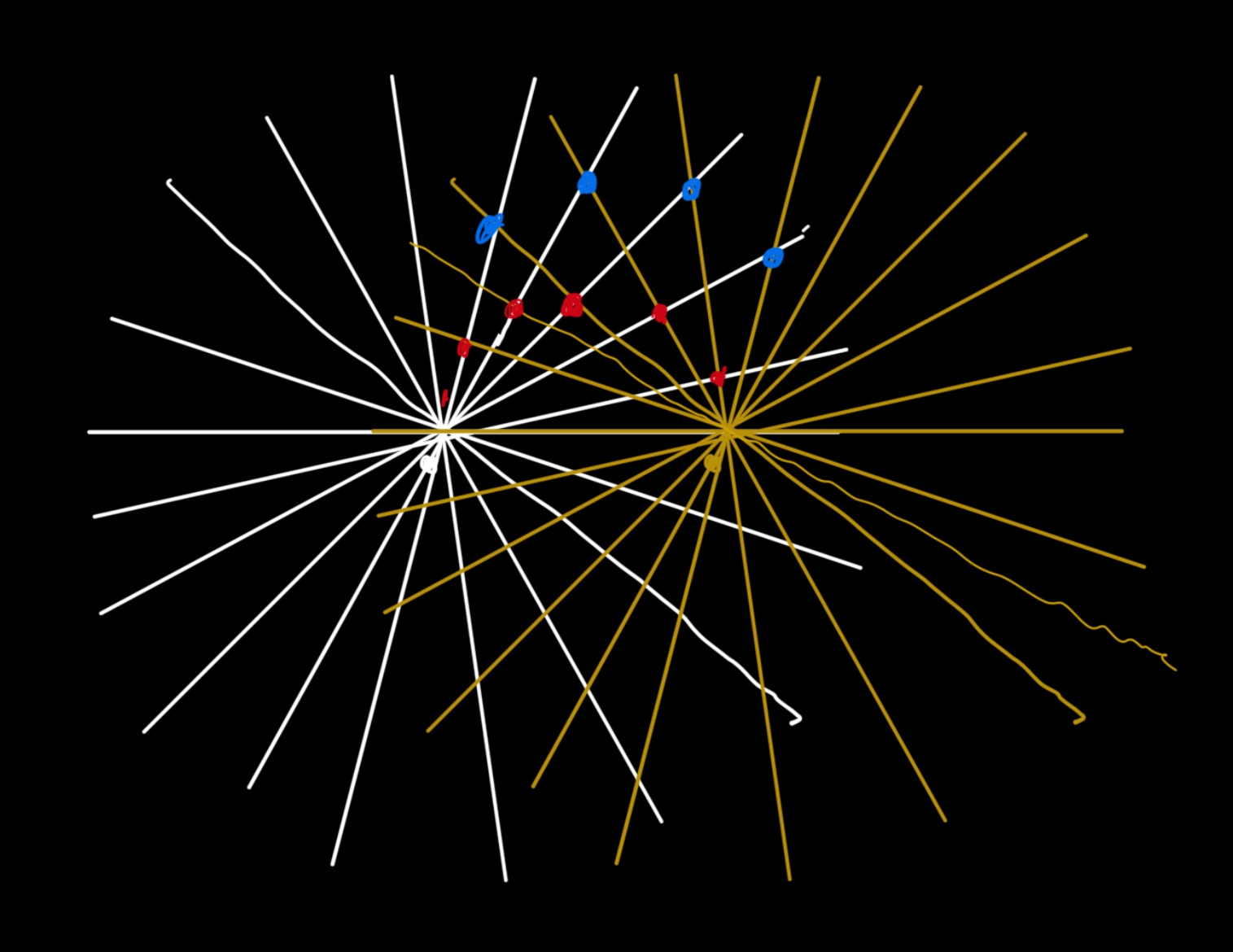
Drawing can only get me so far, but this is an easy enough simulation to do in R, and the results are pretty, especially when we change some of those initial assumptions.

library(ggplot2)
library(purrr)
library(patchwork)
library(ambient)
library(wesanderson)
library(httpgd)
library(ggdark)
library(viridis)
library(fields)
set.seed(12345)

theme_set(
  dark_theme_void() +
    theme(plot.background = element_rect(fill = "#1F1F1F", color = "#1F1F1F"))
)

What’s things do we need for the simplest possible simulation? - two fixed points A and B for our light sources - a way to calculate the angle formed at any other point X where beams from A and B intersect - a way to convert this angle into an intensity value - calculate the intensity for many different points in the plane - visualize the result

Here are some basic functions to do this:

#' Calculates the angle formed by AX and BX
#'
#' @param X A point object representing the origin point.
#' @param A A point object representing the first vector.
#' @param B A point object representing the second vector.
#' @return The angle in radians between vectors A and B with respect to point X.
angle <- function(X, A, B) {
  # restructure for efficiency with many points
  X <- as.matrix(X)
  if (length(X) == 2) X <- t(X)
  A <- rep(A, each = length(X)/2)
  B <- rep(B, each = length(X)/2)

  v1 <- X - A
  v2 <- X - B
  dot_product <- rowSums(v1 * v2)
  norm <- (sqrt(rowSums(v1 * v1)) * sqrt(rowSums(v2 * v2)))
  cos_theta <- dot_product / norm
  acos(cos_theta)
}

#' Convert angle to intensity
#'
#' @param theta A numeric value representing the angle in radians.
#' @return A numeric value representing the intensity.
angle_to_intensity <- function(theta) {
  1 - abs(theta - pi / 2) / (pi / 2)
}


#' Calculate intensity at a point
#' 
#' @param x A point object where the intensity is to be calculated.
#' @param source1 A point object representing the first source point.
#' @param source2 A point object representing the second source point.
#' @param angle_transform_fun A function that takes an angle in radians and returns
#'  a value to be plotted as the coordinate intensity. Default is a linear function of 
#'  the absolute deviation from a right angle.
#' @return A numeric value in [0, 1] representing the intensity at point x.
intensity <- function(x, source1, source2, angle_transform_fun = angle_to_intensity) {
  theta <- angle(x, source1, source2)
  angle_transform_fun(theta)
}

With these functions in hand we can play around. We need two sources:

A <- c(-1, 0)
B <- c(1, 0)

Just as an illustration, the maximum intensity should at a point (0, 1) which forms a right angle. The minimum intensity should be any point on the AB line, e.g. (0, 0) as it forms a 180 degree angle

intensity(c(0, 1), A, B)

[1] 1

intensity(c(0, 0), A, B)

[1] 0

Now we need a grid of points where their beams will intersect:

grid <- expand.grid(
  x = seq(-2, 2, 0.01),
  y = seq(-2, 2, 0.01)
)

and evaluate their intensity:

grid$intensity1 <- intensity(grid[c("x", "y")], A, B)

main <- ggplot(grid, aes(x, y, fill = intensity1, color = intensity1)) +
  geom_raster()
  
main + scale_fill_gradientn(colors = viridis::inferno(256))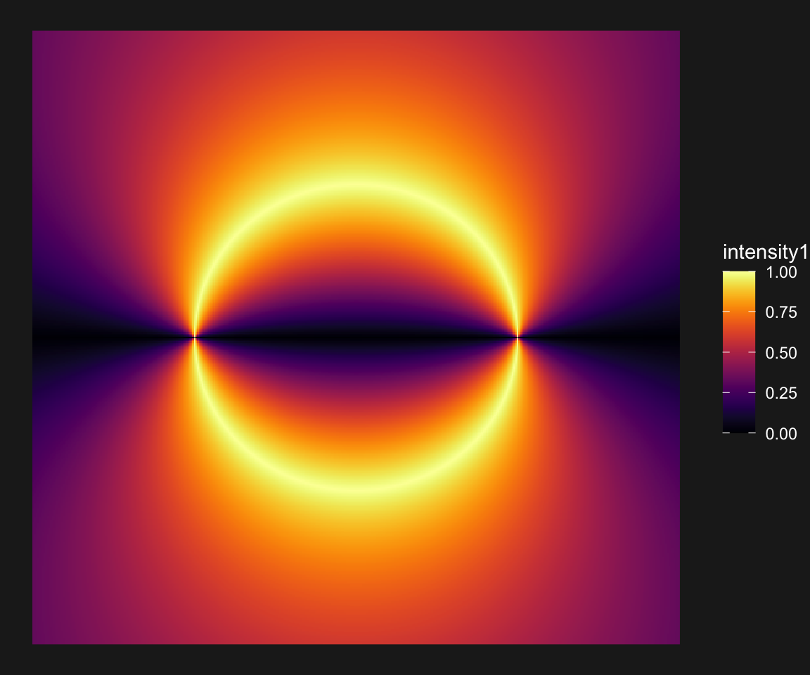

That’s kinda cool. Mostly what I expected, but it’s pretty. We can try a few more pallettes and plot settings. To make things a bit easier, I want to plot multiple granularities with each palette:

plot3s <- function(main, pallette) {
  p1 <- main + 
    scale_fill_stepsn(colors = pallette, n.breaks = 12) + 
    theme(legend.position = "none")
  p2 <- main + scale_fill_stepsn(colors = pallette, n.breaks = 24) + theme(legend.position = "none")
  p3 <- main + scale_fill_gradientn(colors = pallette) + theme(legend.position = "none")
  p1 + p2 + p3
}

For example with out original palette we get:

plot3s(main, viridis::inferno(256))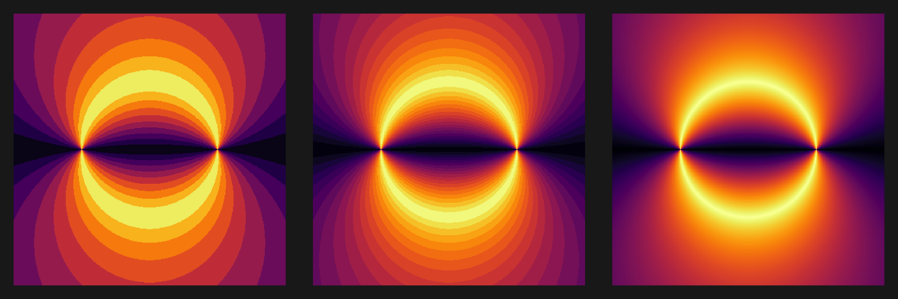

With the binned version on the left I notice something that wasn’t as obvious in the smooth one: There is more than one circle! In fact, all points that form the same angle with A and B lie on a circle. That this would be the case was not at all obvious to me, though eventually I remembered that this is just the inscribed angle theorem from high school geometry. The theorem is a more general case of the more widely known Tales theorem - that all points on a circle form 90 degree angles with any diameter line of the circle. The resulting figure also represents one half of what is known as the Apollonian circles. A well deserved wikipedia rabbit-whole lead to me read more about alternative coordinate systems like the bipolar coordinate system, which at first glance seems esoteric and pointless, but turns out it can simplify many problems that are otherwise too complicated to compute in standard cartesian coordinate systems.

Anyway, let’s go on with making pretty variations on this theme.

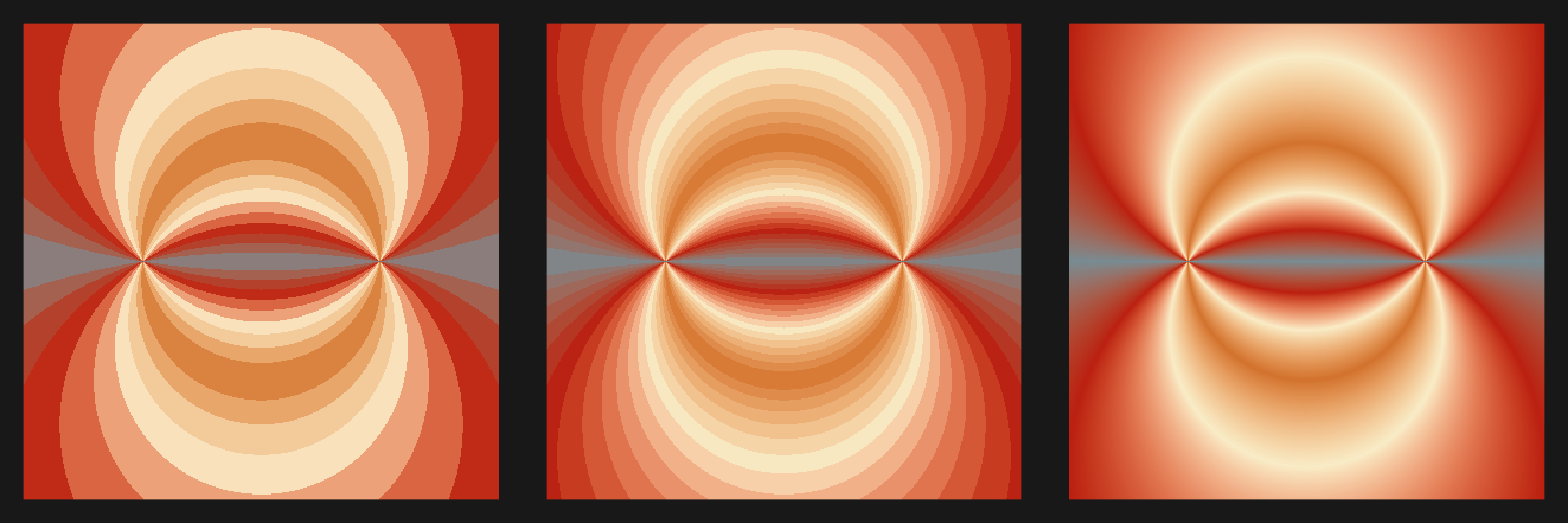
plot3s(main, hcl.colors(12, "YlOrRd", rev = TRUE))
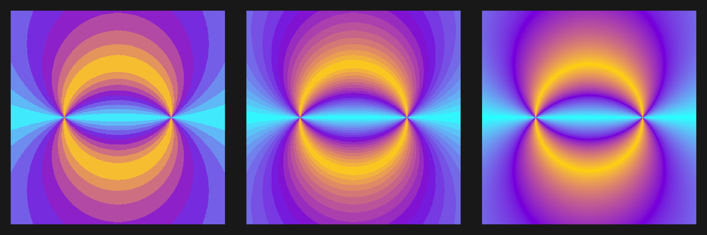
plot3s(main, c("#00FFFF", "#8A2BE2", "#FFD700"))
plot3s(main, wes_palette("Royal1"))

Alright, how about we add some correlated noise for variety?

smooth_matrix_gaussian <- function(mat, sigma = 1) {
  # Create 1D Gaussian kernel
  create_gaussian_kernel <- function(sigma, size = NULL) {
    if (is.null(size)) {
      size <- ceiling(3 * sigma) * 2 + 1 # Ensures kernel covers ~99% of distribution
    }
    x <- seq(-size %/% 2, size %/% 2)
    kernel <- exp(-(x^2) / (2 * sigma^2))
    kernel / sum(kernel) # Normalize
  }

  # Generate 1D Gaussian kernel
  kernel_1d <- create_gaussian_kernel(sigma)

  # Apply separable convolution (first along rows, then columns)
  smooth_rows <- t(apply(mat, 1, function(row) convolve(row, kernel_1d, type = "filter")))
  apply(smooth_rows, 2, function(col) convolve(col, kernel_1d, type = "filter"))
}

# padding because the smoothing kernel drops edges
grid_size <- sqrt(nrow(grid)) + 61 
noise <- matrix(rnorm(grid_size^2), grid_size)
noise <- smooth_matrix_gaussian(noise, sigma = 10)

Now won’t you look at that!

grid$intensity2 <- grid$intensity1 + as.vector(t(noise))

noise_plot <- grid |> 
  ggplot(aes(x, y, fill = intensity2, color = intensity2)) +
  geom_raster() +
  theme(legend.position = "none")

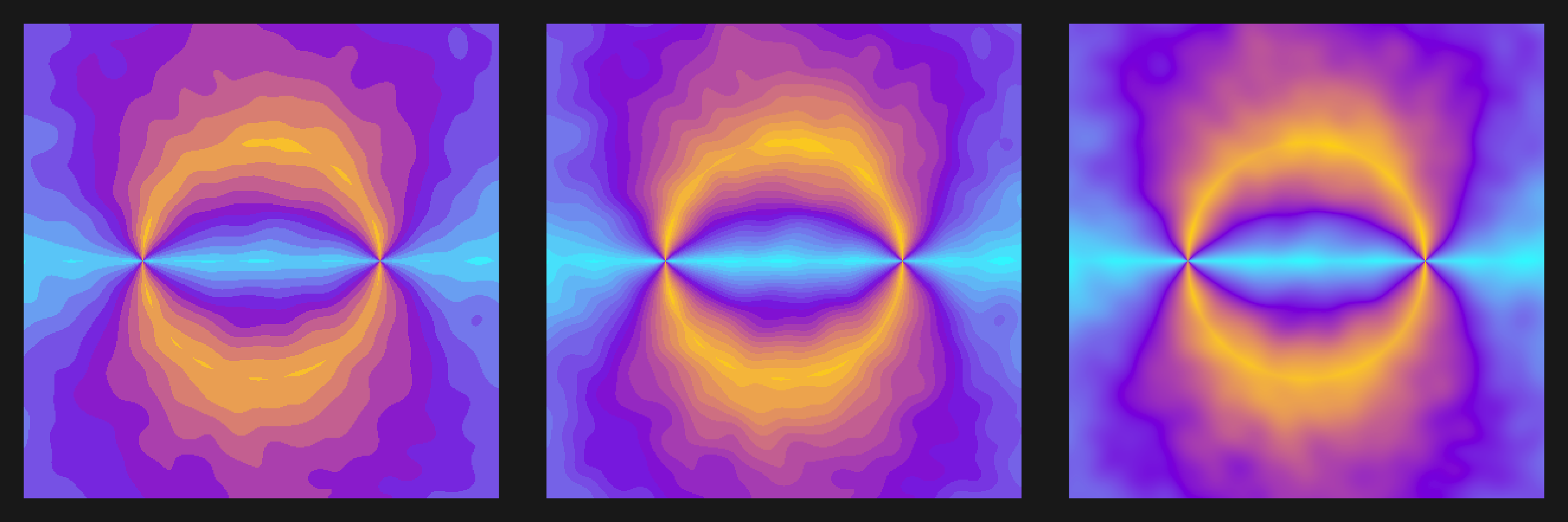
plot3s(noise_plot, rev(viridis::inferno(256)))
plot3s(noise_plot, hcl.colors(12, "YlOrRd", rev = TRUE))
plot3s(noise_plot, c("#00FFFF", "#8A2BE2", "#FFD700"))
plot3s(noise_plot, wes_palette("Royal1"))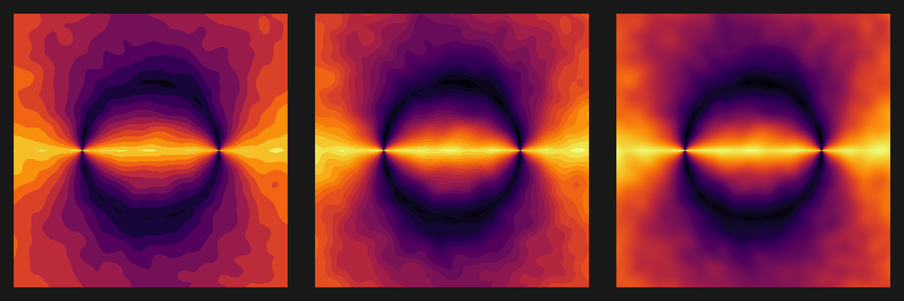

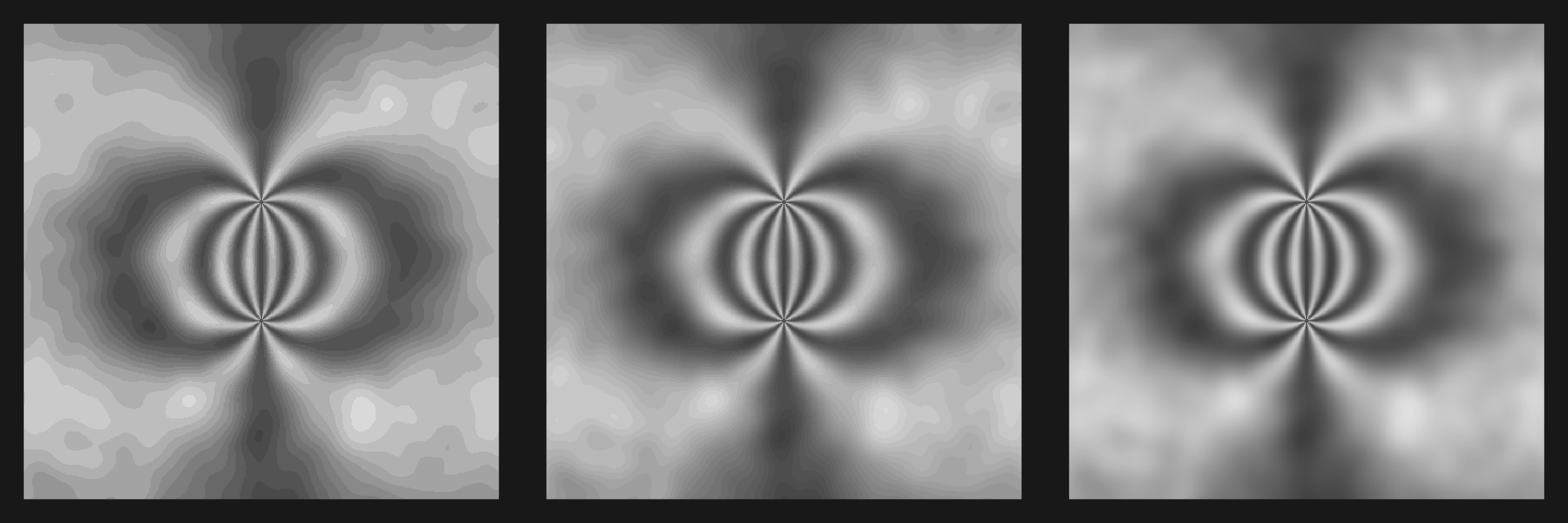
Alright, one last one. Instead of clamping the intensity to be a linear function of how much the angle deviates from 90 degrees, let’s introduce some oscillations:

nonlinear_intensity <- function(theta) {
  deviation <- abs(theta - pi/2) / (pi/2)
  return(sin(2 * pi * deviation)^2)  # Nonlinear transformation
}

bigger_grid <- expand.grid(
  x = seq(-4, 4, 0.02),
  y = seq(-4, 4, 0.02)
)

# padding because the smoothing kernel drops edges
bigger_grid_size <- sqrt(nrow(bigger_grid)) + 61 
bigger_noise <- matrix(rnorm(grid_size^2, sd = 2), bigger_grid_size)
bigger_noise <- smooth_matrix_gaussian(bigger_noise, sigma = 10)

bigger_grid$intensity3 <- intensity(bigger_grid[c(1,2)], A, B, nonlinear_intensity) + as.vector(t(bigger_noise))

noise_plot_nl <- bigger_grid |> 
  ggplot(aes(y, x, fill = intensity3, color = intensity3)) +
  geom_raster() +
  theme(legend.position = "none")

plot3s(noise_plot_nl, viridis::inferno(256))
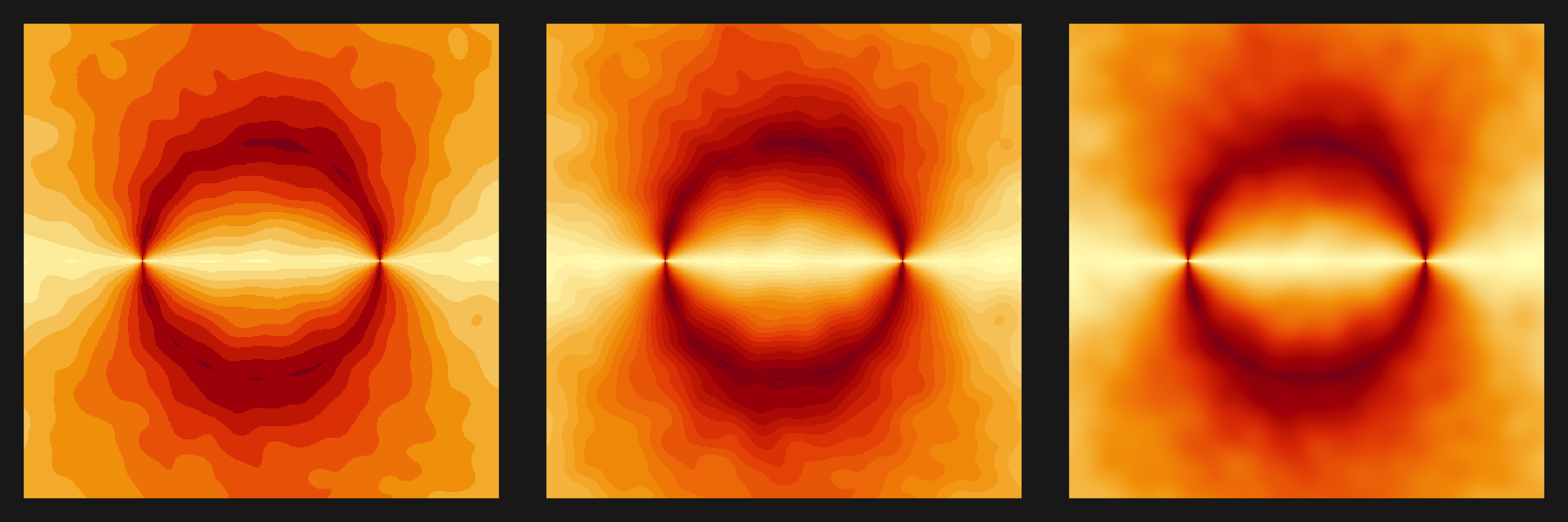
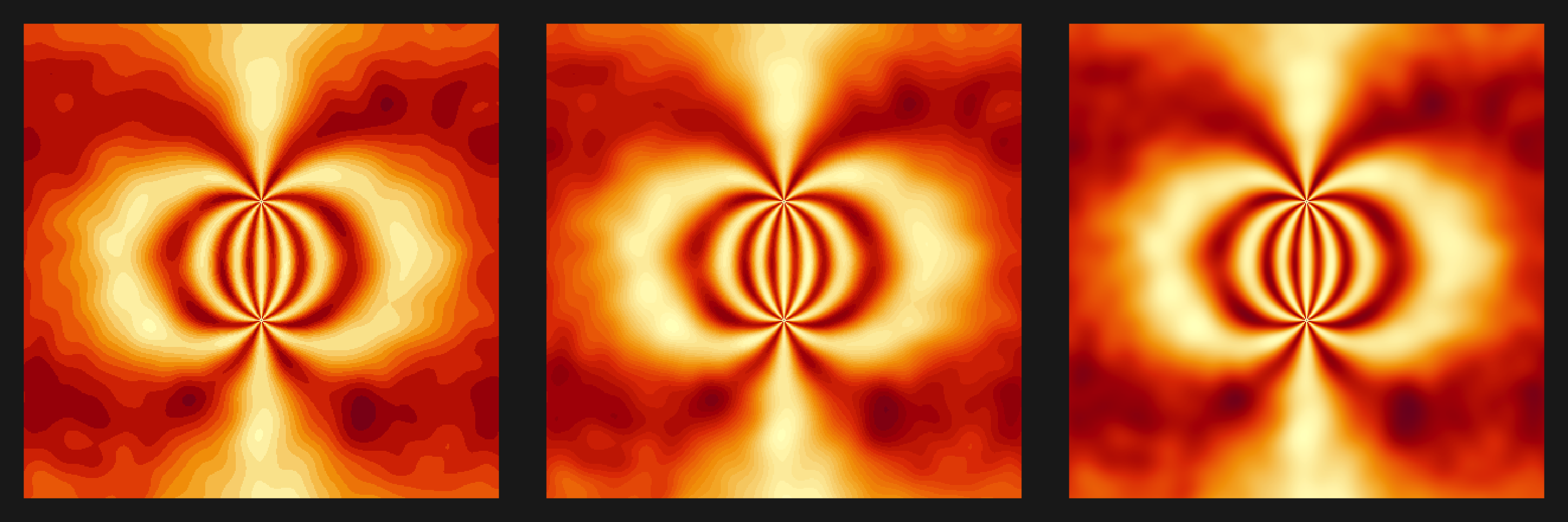
plot3s(noise_plot_nl, hcl.colors(12, "YlOrRd", rev = TRUE))
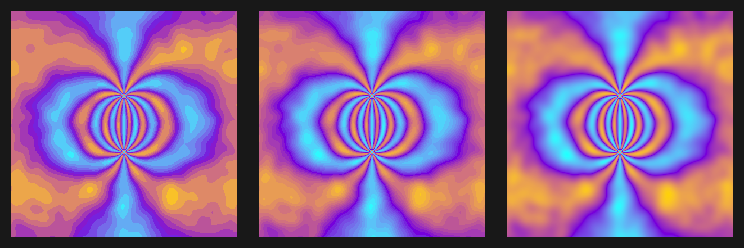
plot3s(noise_plot_nl, c("#00FFFF", "#8A2BE2", "#FFD700"))
plot3s(noise_plot_nl, grey.colors(2))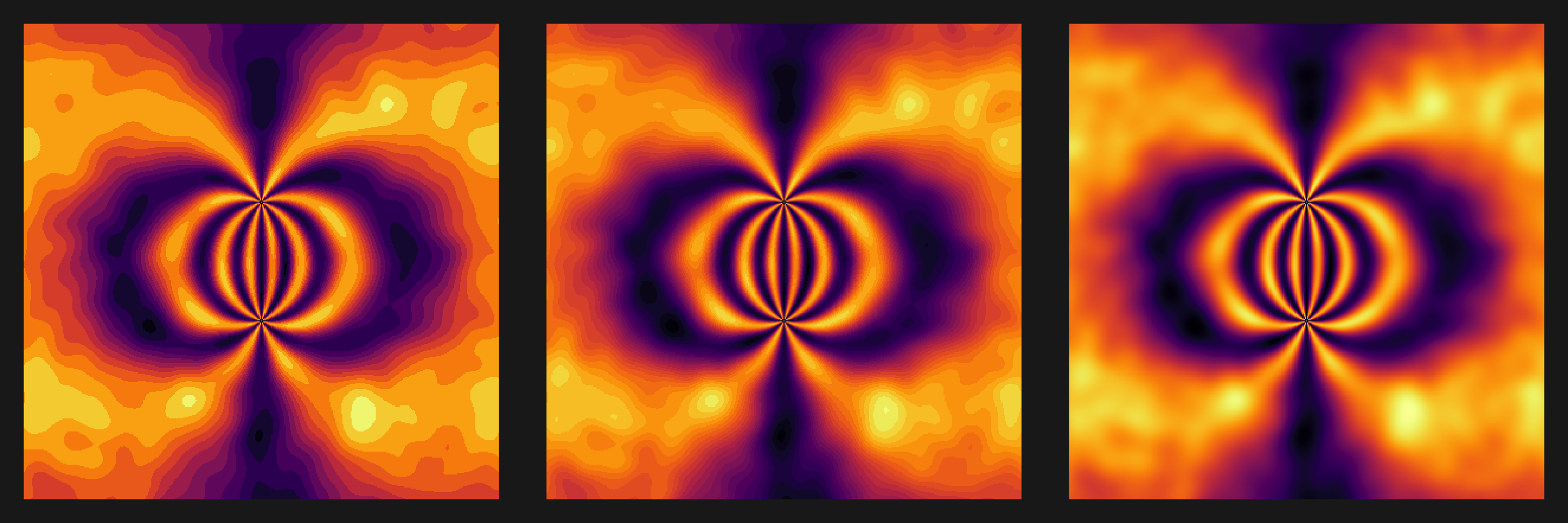

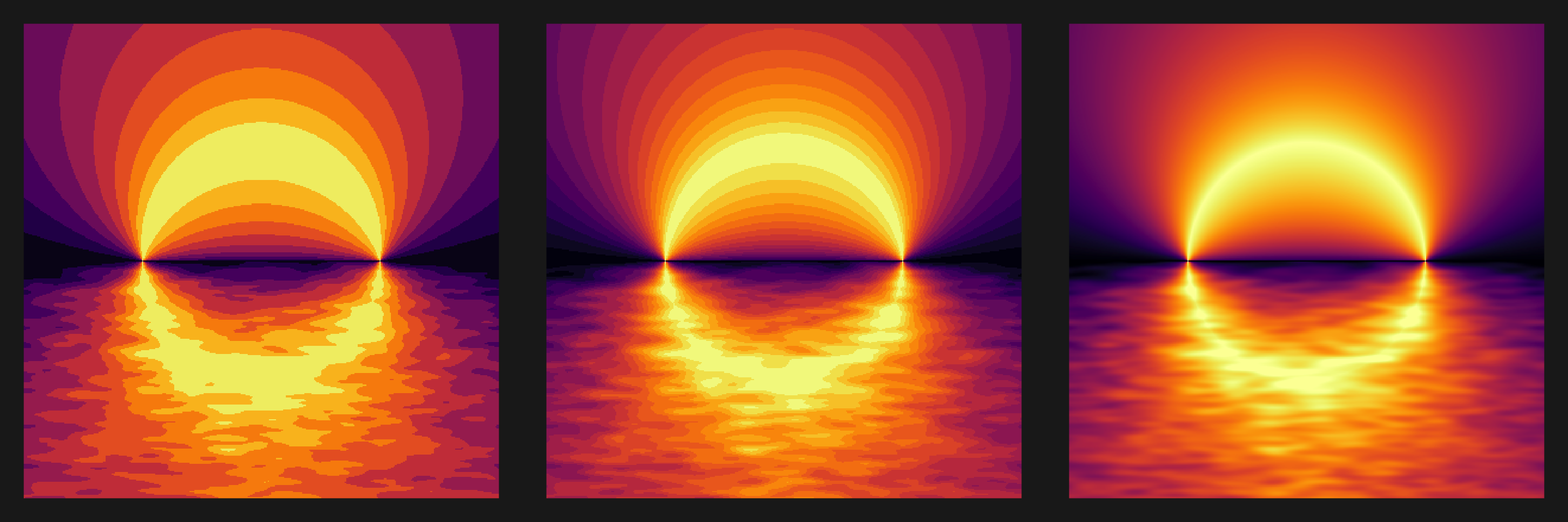
Last for real this time:

streak_noise <- function(mat, sigma_x = 10, sigma_y = 3) {
  size_x <- ceiling(3 * sigma_x) * 2 + 1
  size_y <- ceiling(3 * sigma_y) * 2 + 1
  
  kernel <- outer(-size_x:size_x, -size_y:size_y, function(x, y) {
    exp(-(x^2 / (2 * sigma_x^2) + y^2 / (2 * sigma_y^2)))
  })
  kernel <- kernel / sum(kernel)  # Normalize kernel
  
  # Pad kernel to match matrix size
  pad_kernel <- matrix(0, nrow = nrow(mat), ncol = ncol(mat))
  kx <- floor(nrow(kernel) / 2)
  ky <- floor(ncol(kernel) / 2)
  pad_kernel[1:nrow(kernel), 1:ncol(kernel)] <- kernel
  
  convolve2d <- function(mat, kernel) {
    fft_mat <- fft(mat)
    fft_kernel <- fft(kernel, dim(mat))
    return(Re(fft(fft_mat * fft_kernel, inverse = TRUE) / length(mat)))
  }
  
  return(convolve2d(mat, pad_kernel))
}

# Generate and smooth directional noise
grid_size <- sqrt(nrow(grid))
noise_matrix <- matrix(rnorm(grid_size^2), nrow = grid_size)
smoothed_noise <- streak_noise(noise_matrix, sigma_x = 10, sigma_y = 2)

# Normalize and scale noise
smoothed_noise <- (smoothed_noise - min(smoothed_noise)) / 
                  (max(smoothed_noise) - min(smoothed_noise)) * 0.3 - 0.15

# Apply noise and clip values
lower_part <- grid$y < 0
grid$intensity4 <- ifelse(
  lower_part,
  pmax(pmin(grid$intensity1^0.75 + as.vector(smoothed_noise), 1), 0),
  grid$intensity1
)
inside_upper_circle <- (grid$y^2+grid$x^2 <= 1) & (grid$y >= 0 )
grid$intensity4[inside_upper_circle] <- grid$intensity4[inside_upper_circle]^0.4

sterak_noise <- grid |> 
  ggplot(aes(x, y, fill = intensity4, color = intensity4)) +
  geom_raster() +
  theme(legend.position = "none")

plot3s(sterak_noise, viridis::inferno(256))